How to use pivot table to group same item data and calculate sum, count, average, max, min in Ms Excel 2013

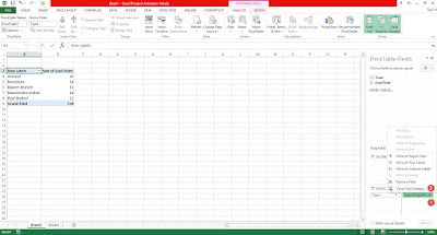
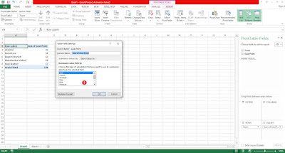
The pivot table will automate how to calculate sum, count, average, max, min, standard deviation etc based on data group which are associated to the same data. This make the analysis work / calculation easier and faster to achieve without manually group them. The pivot table also have a filter that allow users to filter the data group which they want to display only.

In order to use the pivot table Ms Excel 2013

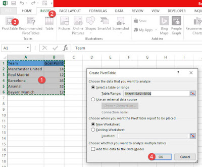
1. Select the data you want to analyze including its header
2. Select INSERT>Pivot Table
3. It will prove which data to analyze just click OK since it is already selected
4. Select the field you want to display in pivot table
5. Put numbers in the values section which you want to analyze sum, count, average, max or min

You can also analyze percentage data

Clear cells format in MS EXCEL 2013

Copy and Paste data from format i.e. CSV, HTML, Words, etc carried over the format that you don't want in excel. However that can be solved by removing / clear the formatting of the data in the excel itself. This tip is based on Ms Excel 2013.

All kind of format can be removed: Colors, Font Size, Font Format (italic, bold, superscript, subscript), Font type, etc. Clear all formatting will clear all the format and reset it to default.

1. Select the cells that you want to clear its format. Multiples selection of cells are allowed
2. Go to Home> Clear > Clear Format



You can also clear comments, hyperlink, and contents of the cells